1 Methods
All scripts (as well as raw data, results, and this document) are available on GitHub(Finnerty 2021).
1.1 Datasets
A list of PDBs was assembled that represented either a representative sample of a variety of proteins, with a resolution better than 3A, (HEM and HEC) or, all proteins containing these ligands were downloaded from the PDB (in the case of SRM, VER, VEA). Not all downloaded PDBs were appropriate for this study (e.g. contained superimposed structures) and therefore the amount of PDBs was culled. The datasets are current as of 16 August 2021.
The size of the datasets actually used in the study were as follows: HEM (n=58), HEC(n=13), SRM (n=9), VER (n=2) and VEA (n=2), which are merged for a combined n=4 for VERDOHEME.
The name of all proteins used in the study and their source organism are provided tables within Appendix B.1.
1.2 Pre-processing
Many of the PDBs downloaded were multimeric structures. The number of subunits per protein would skew results and overrepresent especially large multimeric proteins. Therefore, to only allow for one heme binding site per PDB, all downloaded PDBs were converted to monomeric structures. This was achieved by saving a single chain (chain A) of each PDB and eliminating all other chains. The single chain was then saved as a PDB and used in all subsequent scripts. Part of the script is reproduced below:
from chimera import runCommand as rc
# select chain A, a single unit
rc("sel :.a")
# select everything else
rc("sel invert sel")
# delete everything else besides that chain A
rc("del sel")
# now save the monomer:
rc(("write format pdb 0 "+unexpandedResultPath+activeLigand+"/%s")%
  (fn + ".mono.pdb"))
1.3 Processing Monomers
UCSF-Chimera was used to generate all data in this study. Multiple Python scripts were employed to achieve a high-throughput process where all monomeric PDBs could be processed in the same session.
Chimera was used to predict the following qualities: Volume of the ligand binding pocket, accessible and excluded surface area of the ligand, and accessible and excluded surface area of the binding pocket. These calculations require a population of atoms to be selected for the calculation.
Atoms were selected within a distance cutoff, to be considered as potentially interacting with the ligand or forming the binding pocket. Distance cutoffs from the ligand of 5A and 7A were chosen; for the predicted qualities, the algorithms were run twice to get values at 5A and 7A. For the distance and angle calculations, only the 7A distance cutoff was used, as the cutoff does not factor into any calculations and may be set during analysis.
As these cutoffs are selected arbitrarily, data from the 5A and 7A runs are overlaid in the figures reported in Appendix A. Data tables are also provided in Appendix B.
1.3.1 Amino Acid Frequency
Amino acids within the bounds of the lower and upper distance cutoff were selected and recorded. These were then counted for frequency per residue.
1.3.2 Volume Calculations
Volume of the binding pocket was predicted via Surfnet (Laskowski 1995), and run with default parameters of Grid Interval = 1.0 and Distance Cutoff = 10.0 (the latter option does not relate to the distance cutoff from the ligand). Surfnet is the molecular volume calculation tool implemented within UCSF Chimera. The script used selects the residues around heme to consider as the bounds of the pocket, but effectively ignores heme’s presence as its calculates the volume, as if the pocket were empty:
from chimera import runCommand as rc
# Select the atoms within 7A of heme.
#Then, of that selection, keep everything but heme.
rc("sel :"+activeLigand+" za < "+angstromDistance)
# this is the syntax that accomplishes our desired selection
rc("sel sel &~:"+activeLigand)
interface_surfnet("sel","sel")
rc("sop split #") # acquire the individual pockets that have been generated
rc("measure volume #") # measures volume of individual pockets
# in R we keep only the largest volume
Surfnet, at least in this investigation, was prone to generating very small volumes. During analysis these were removed and only the largest volume generated is recorded, since the largest volume generated and identified is most likely the binding pocket. Two figures below demonstrate a run where one good pocket is produced, and one where a few very small “bubbles” are generated:
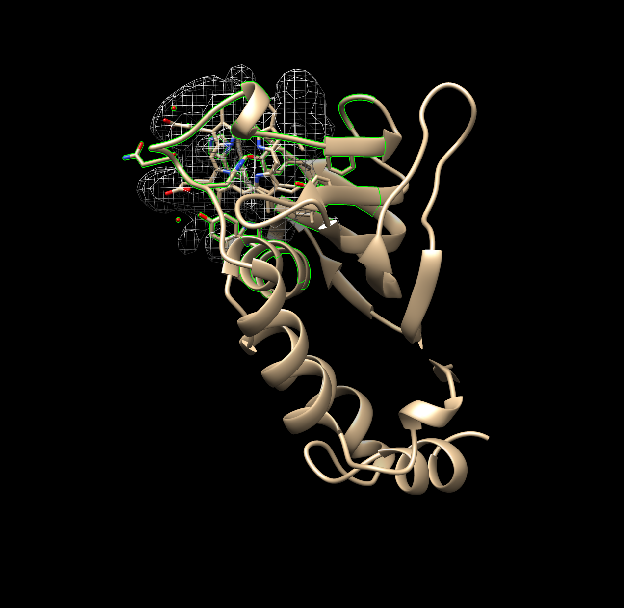
Figure 1.1: Good Example of Surfnet Run (1B2V)
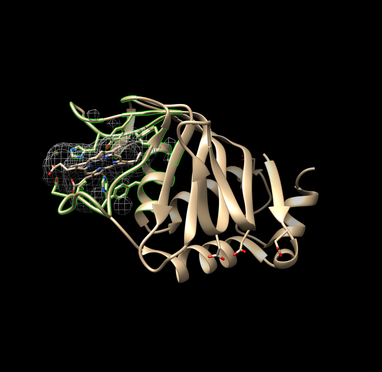
Figure 1.2: Non-Ideal Example of Surfnet Run (1DKH)
1.3.3 Surface Area Calculations
Solvent excluded and solvent accessible surface areas of both the ligand and the binding pocket were calculated using Chimera’s “surf” algorithm, which itself is an implementation of a program called MSMS (Sanner, Olson, and Spehner 1996).
These two measures are similar but not the same. Solvent accessible surface area represents the surface area of the protein that a solvent molecule (i.e. water) may interact with. It is calculated by rolling a sphere on the Van der Waals surface of the protein, and the center of the sphere is recorded as the bounds of the accessible surface area. Solvent excluded surface area is calculated the same way, rolling a sphere on the Van der Waals surface of the protein, but instead the point of contact of the sphere against the Van der Waals surface is recorded as the excluded surface area. The solvent excluded surface area may therefore be considered the bounds of the protein itself, versus the solvent accessible surface area, which can be considered the bounds at which a solvent may interact with the protein(Sanner, Olson, and Spehner 1996).
1.3.4 Distance Calculations
Distances of amino acids from the ligand could not be calculated accurately nor precisely in a direct way. Instead, distances for each atom composing a residue were calculated. This was achieved using a built-in function of chimera; the syntax is not straightforward, but part of the script is shown below. The distances of all atoms within a residue were averaged, and this value was taken as the mean distance of the entire residue and used in subsequent steps.
from chimera import runCommand as rc
#select and define the Fe atom
rc("sel :HEM@Fe")
# index to acquire the one atom selected
fe = chimera.selection.currentAtoms()[0]
# select all atoms within angstromDistance of Fe (also de-selects Fe)
rc("sel sel za < "+settings.angstromDistance)
# define this selection of atoms within distance as a list
nearbyAtoms = chimera.selection.currentAtoms()
# parse and print the distances (and coordinates) of these atoms
for i in nearbyAtoms:
  print "Atom being analyzed...", i, "... Distance to Fe...",
  #prints distance between atom i and the Fe atom
  i.coord().distance(fe.coord())
The data produced in this step therefore include the mean distance of each amino acid. Distances are traceable per residue and atoms in each residue; this data was used to construct the distributions of amino acids over distance, and the angular data below are cross-referenced with this list of distances.
1.3.5 Planar Angle Calculations
Individual residues and the ligand were defined as axes. The angle between each residue’s axis and the axis of the ligand were calculated. Each axis functions essentially as a separate plane. This employed the “define axis,” and “angle” functions of Chimera; the Axes/Planes/Centroids Structural Analysis function of Chimera via GUI.
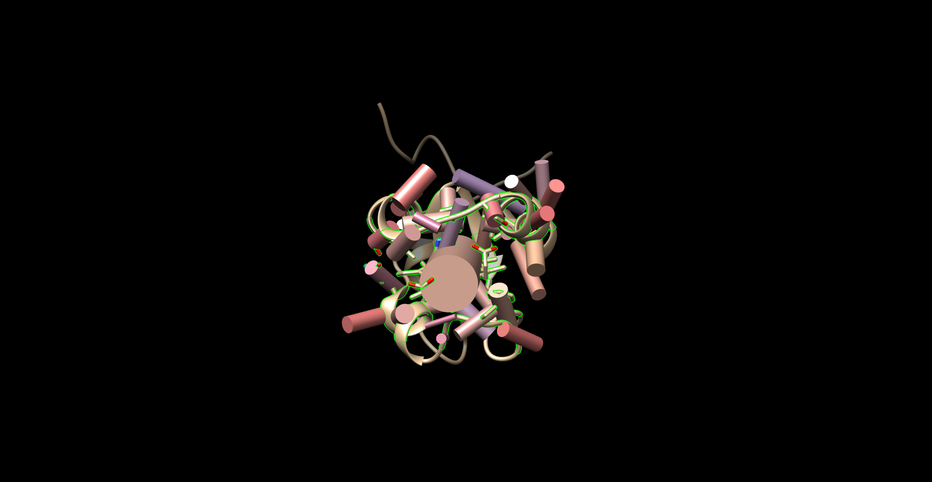
Figure 1.3: Example of Planar Angles Calculation (1B5M)
1.3.6 CA-CB-Fe Calculations
Residues within the distance cutoff were examined one by one. The angle of between each residue’s carbon alpha (CA) and carbon beta (CB) and the Fe of the ligand was calculated, using the “angle” function of Chimera. The ligand nor the Fe atom were compared with themselves.